Baris 11 membentuk layer ke 1 dengan 2 unit dense, dimana inputnya adalah 1, yaitu x
Baris 12 membentuk layer ke 2 dengan 1 unit dense
Baris 13 membentuk model dalam bentuk sequensial (berurutan) dari layer ke-1 dilanjutkan layer ke-2
Baris 14 membuat model training menggunakan optimizer SGD (Stochastic Gradient Descent), sedangkan lost function-nya (untuk mengurangi kesalahannannya) menggunakan metode Mean Square Error (MSE). Lihat di Machine Learning #1 untuk lebih jelasnya
Selanjutnya lakukan training 50 kali, sesuai perintah di baris 19
Hasil nilai w dan b di setiap dense adalah berikut:
Pada layer ke-1, dense 1: w=0,9896864 dan b=-1,0169075 sedangkan dense 2: w=-0,38317692 dan b=0,24202025
Pada layer ke-2, dense: w1=0,8393119; w2=-1,0042762; b=0,06092146
Hasil prediksinya saat nilai x 4 adalah 6,90 yang sudah lebih mendekati angka 7, dibandingkan dengan di Machine Learning #1 yang hasilnya 6,80
Jika ada nilai input: x = [-1 0 1 2 3 4] ternyata menghasilkan nilai ouput: y = [-3 -1 1 3 5 7]
Jadi, apa rumus dari y ? apakah y=2x+1 atau y=x-2 atau yang lainnya?
Mari kita ajarkan nilai input dan ouput ini ke “MESIN”, agar si MESIN ini bisa belajar mencari model matematikanya. Dalam hal ini kita sebut saja dengan Machine Learning.
MESIN kita berikan petunjuk bahwa rumus dari y adalah linier, (y = wx + b) dimana w dan b adalah bilangan yang harus dicari oleh mesin.
Anggap saja Mesin menebak, w=3 dan b=-1, (y = 3x – 1) namun ternyata dari hasil perhitungan rumus itu adalah y = [-4 -1 2 5 8 11]
Hijau => Tebakan Mesin, Biru => Nilai seharusnya
Selisih dari setiap elemen perhitungan adalah, gap = [-1 0 1 2 3 4]
Jika setiap selisih dikuadratkan, maka gap = [1 0 1 4 9 16]
Jumlah dari kesalahan gap adalah, err = 1 + 0 + 1 + 4 +9 +16 = 31. OK, bagaimana kalau diakarkan saja? gap-nya kan dikuadratkan, jadi agar sebanding maka err adalah akar dari 31. Ini disebut dengan Mean Square Error, MSE = 5,57 (atau akar dari 31).
Ok, mesin coba jika y = 2x – 2. Maka hasil perhitungannya, y = [-4 -2 0 2 4 6], kalau dihitung MSE-nya maka hasilnya adalah 1 (MSE= 2,23) Wow, MSE sudah mulai berkurang. Proses ini dilakukan berulang ualng.
Mesin mencoba lagi, y = 2x – 1. Maka hasil perhitungannya y = [-3 -1 1 3 5 7] nah… ini baru tepat!
Mesin berhasil menebak, rumus matematikanya adalah y = 2x – 1
Menerapkan analogi di atas pada Machine Learning lewat Colabs (Atau jupyter notebook)
import tensorflow as tf
import numpy as np
from tensorflow import keras

model = tf.keras.Sequential([keras.layers.Dense(units=1, input_shape=[1])])
model.compile(optimizer='sgd', loss='mean_squared_error')

x = np.array([-1.0,  0.0, 1.0, 2.0, 3.0, 4.0], dtype=float)
y = np.array([-3.0, -1.0, 1.0, 3.0, 5.0, 7.0], dtype=float)

model.fit(x, y, epochs=50)
Baris 1 – 3 adalah penggunaan library tensonflow, numpy dan keras.
Baris 5, kita membuat model 1 input dan 1 output.
Baris 6, kita gunakan optimizer SGD (Stochastic Gradient Descent), sedangkan lost function-nya (untuk mengurangi kesalahannannya) menggunakan metode Mean Square Error (MSE) seperti yang dianalogikan di atas.
Baris 8 adalah nilai masukan, sedangkan baris 9 adalah hasil ouputnya.
Baris 10, kita minta MESIN untuk mencari model matematikanya dengan mencobanya sebanyak 50 kali.
Pertama tama, w=3 dan b = 1, namun error (loss) nya adalah 15,1. Karena gradien dari loss sudah ditemukan, maka MESIN mulai mengubah w dan b sesuai arah gradien, dalam hal ini percebaan kedua w=1,53 dan b = 0,37. Proses berulang-ulang hingga mencapi perulangan (epoch) yang kita tentukan. Contoh dalam kode ini adalah 50 epoch.
Pada akhirnya di-epoch ke 50, ditemukan w=2 dan b = -0.99 dimana loss-nya mendekati 0 (0,00009)
Perkiraan w dan b oleh MESIN dari epoch 1 hingga 50
Saat ini MESIN yakin bahwa rumus matematika yang didapatkan adalah y = 2x – 0,99 selanjutnya mari kita coba jika x adalah 4.
print(model.predict([4]))
Kode diatas adalah untuk memeriksa, memprediksikan, jika x = 4 maka berapakah nilai y nya
Hasilnya adalah 6.8087044, walaupun seharusnya hasilnya adalah 7
hasil perhitungan MESIN mendekati benar, dari setiap elemen nilai x
Kode untuk menampilkan plot
import tensorflow as tf
import numpy as np
import matplotlib.pyplot as plt

# Tebakan awal
INITIAL_W = 3.0
INITIAL_B = 1.0

# Fungsi menghitung loss
def loss(predicted_y, target_y):
  return tf.reduce_mean(tf.square(predicted_y - target_y))

# Proses training
def train(model, inputs, outputs, learning_rate):
  with tf.GradientTape() as t:
    current_loss = loss(model(inputs), outputs)
  # mencari arah gradien loss
  dw, db = t.gradient(current_loss, [model.w, model.b])
  # perbaiki model untuk epoch berikutnya dengan mengubah w dan b berdasarkan learning_rate
  model.w.assign_sub(learning_rate * dw)
  model.b.assign_sub(learning_rate * db)
  return current_loss

# Mendefinisikan model regresi linier
class Model(object):
  def __init__(self):
    # Inisialisasi w dan b
    self.w = tf.Variable(INITIAL_W)
    self.b = tf.Variable(INITIAL_B)

  def __call__(self, x):
    return self.w * x + self.b

"""Proses Training"""

# tentukan input, output dan learning rate
xs = [-1.0, 0.0, 1.0, 2.0, 3.0, 4.0]
ys = [-3.0, -1.0, 1.0, 3.0, 5.0, 7.0]
LEARNING_RATE=0.09

# Instantiate model
model = Model()

# Menampilkan w, b dan loss di setiap epoch
list_w, list_b = [], []
epochs = range(50)
losses = []
for epoch in epochs:
  list_w.append(model.w.numpy())
  list_b.append(model.b.numpy())
  current_loss = train(model, xs, ys, learning_rate=LEARNING_RATE)
  losses.append(current_loss)
  print('Epoch %2d: w=%1.2f b=%1.2f, loss=%2.5f' %
        (epoch, list_w[-1], list_b[-1], current_loss))

"""### Plot hasil training"""

# Plot nilai w dan b perkiraan dari hasil training terhadap w dan b seharusnya
TRUE_w = 2.0
TRUE_b = -1.0
plt.plot(epochs, list_w, 'r', epochs, list_b, 'b')
plt.plot([TRUE_w] * len(epochs), 'r--', [TRUE_b] * len(epochs), 'b--')
plt.legend(['w perkiraan', 'b perkiraan', 'w seharusnya', 'b seharusnya'])
plt.show()
Papan Arduino NANO 33 BLE Sense dirancang untuk solusi hemat daya dan hemat biaya bagi pembuat piranti elektronika yang memiliki konektivitas Bluetooth Hemat Energi. Menggunakan modul NINA B306, terdiri dari chip mikrokontroler Cortex M4F besutan Nordik, yaitu nRF52480. Arduino NANO 33 BLE Sense sama dengan Arduino NANO 33 BLE namun dengan tambahan satu set sensor yang sangat populer untuk mempelajari Machine Learning sebagai bagian dari kecerdasan buatan atau Artificial Inteligence (AI).
Untuk menggunakan modul ini, perlu menambahkan pustaka (library) Arduino nRF528x mbed Core. Caranya dengan memilih menu Tools, kemudian Boards dan Boards Manager, seperti yang didokumentasikan di halaman Arduino Boards Manager.
Arduino NANO 33 BLE Sense adalah variasi perangkat keras dari Arduino NANO 33 BLE; kedua modul tersebut dikenali sebagai Arduino NANO 33 BLE dan ini normal.
menginstal Driver untuk Arduino NANO 33 BLE Sense.
Dengan nRF528x mbed core diinstal, saatnya melanjutkan dengan penginstalan driver.
Pada Windows, jika menginstal Core nRF528x mbed dengan benar, cukup hubungkan Arduino NANO 33 BLE Sense ke komputer dengan kabel USB. Windows akan memulai proses instalasi drivernya setelah papan dicolokkan.
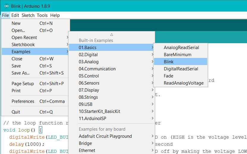
Memulai contoh sketch: blink
Pilih jenis board yang benar
Pilih Port yang sesuai
Mikrokontroler pada Arduino NANO 33 BLE Sense berjalan pada 3.3V, yang berarti tidak boleh menggunakan lebih dari 3.3V ke pin Digital dan Analognya. Berhati-hatilah saat menghubungkan sensor dan aktuator untuk memastikan bahwa batas 3,3V ini tidak pernah terlampaui. Menghubungkan sinyal tegangan yang lebih tinggi, seperti 5V yang biasa digunakan dengan papan Arduino lainnya, akan merusak Sense Arduino NANO 33 BLE.
Tegangan kerja 5V sekarang hanya menjadi pilihan tambahan untuk berbagai modul, sedangkan tegangan 3,3V menjadi tegangan standar untuk IC elektronik.
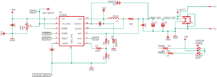
Here is a practical example of shunt resistor selection for an MPPT based solar charge controller circuit. The below circuit uses LT3652, an MPPT charge controller from Linear Technology (Analog devices). However, If we look carefully, the battery that will be charged through this circuit is the load.
The load is connected using a shunt resistor R6. The R6 will determine the charge current, which means the voltage drop of this R6 will remain constant in every case as V = I x R. The R will be constant, the V will be constant, the driver will change the charge current.
To select the shunt resistor, the following things will be required-
The constant voltage that will be used by the driver IC LT3652
The maximum charge current that is required to be delivered to the battery through the resistor.
Since it is a charge controller tolerance could be 1%.
As per the LT3652 datasheet, the sense pin will use 100 mV (0.1V) sense voltage that will be constant. Also, the maximum charge current LT3652 supports is 2A. Thus, the Shunt Resistor value needs to be R = V / I or Shunt resistor value will be 0.1V / 2A = 0.05 Ohms or 50 mili-ohms.
The power rating of this resistor needs to be P = I2R or P = 22 x 0.05 = 0.2 Watt. The close value of the shunt resistor will be 50 mili-ohms, 1% rated, 0.25 Watt. But instead of 0.25 Watt, 0.375 Watt is the safe resistor wattage that can be used.
An issue is that you have to make decisions about how fast a track is moving under pure signals from a single pot and what to do when signals from the other pot are included. For example, if you push the FB (Forward-Backward pot fully forwards, and if both motors then run at full speed ahead, how do you deal with the addition of a small amount of LR (Left-Right) pot being added. To get rotation you have to have one track going faster that the other. So, if you are already running at maximum forwards speed on both motors you must decrease one or other track speed in order to turn. But, if you had been standing still you would have accelerated one or other track to achieve the same result.
So, all that said, here is a simple off-the-cuff starting solution out of my head which seems like good start.
If pots are mechanically independant then both can be at 100% simultaneously. If both are on a joystick type arrangement, if Yaxis = 100% and Xaxis = 0%, then adding some B will usually reduce A. A joystick could be constructed where the above is not true, but these are unusual. Assume that the joystick is of the type that increasing Y% when X = 100% will reduce X. Other assumptions can be made.
FB = front-back pot. Centre zero, +Ve for forward motion of pot
LR = Left right pot. Centre zero. +Ve for pot at right.
K is a scale factor initially 1. If any result exceeds 100% then adjust K so result = 100% and use same K value for other motor also.
eg if Left motor result = 125 and Right motor result = 80 then. As 125 x 0.8 = 100, set K = 0.8. Then. Left = 125 x 0.8 = 100%. Right = 80 x 0.8 = 64%.
Then:
Left motor = K x (Front_Back + Left_Right)
Right motor = K x (Front_Back – Left_Right)
Sanity checks:
LR = 0 (centered), FB = full fwd -> Both motors run full forwards.
LR = full left, FB = 0 -> Left motor runs full backwards, Right motor runs full forwards. Vehicle rotates anti clockwise.
FB was 100%, Lr = 0%. Add 10% of LR to right. L = FB+LR = 100%- + 10% R = FB-LR = 100%- – 10%
If largest axis < 100%, scale until = 100%. Then scale other axis by same amount.
Looking at highly price Camera SDK to handle ONVIF Standard, I decided to build some code to control PTZ camera movement using C#.
It it a nice tutorial video by Onvif Channel. That video describes basic step to make a C# project on visual studio. Unfortunately, I can’t get it work for my camera. I’m having YooSee camera GW-1113 which is already support PTZ Control.
There is another tutorial in CodeProject to use PTZ Control. My code is always get a closed connection message from the camera. Both using password or nor, it alway failed. Next, I got nice tool to cek my Onvif Camera. It can detect camera’s IP, port, display video stream and controlling camera using PTZ. You can get it here https://sourceforge.net/projects/onvifdm/ Afterward, I got IP, Port, and service.
With correct IP, Password, port and service address, it still error on getProfiles() command. I inisiate to find tool to debug Onvif request. I grab this tool in this forum https://support.yooseecamera.com/threads/233/ Nice step by step tutorial with pictures. I made my dummy service and dump post header request and then save it into textfile. Here is PHP code i got from // https://gist.github.com/magnetikonline/650e30e485c0f91f2f40 to dump request. I save it on http://localhost:5000/onvif/device_service/index.php
<?php

class DumpHTTPRequestToFile {

	public function execute($targetFile) {

		$data = sprintf(
			"%s %s %s\n\nHTTP headers:\n",
			$_SERVER['REQUEST_METHOD'],
			$_SERVER['REQUEST_URI'],
			$_SERVER['SERVER_PROTOCOL']
		);

		foreach ($this->getHeaderList() as $name => $value) {
			$data .= $name . ': ' . $value . "\n";
		}

		$data .= "\nRequest body:\n";

		file_put_contents(
			$targetFile,
			$data . file_get_contents('php://input') . "\n"
		);

		echo("Done!\n\n");
	}

	private function getHeaderList() {

		$headerList = [];
		foreach ($_SERVER as $name => $value) {
			if (preg_match('/^HTTP_/',$name)) {
				// convert HTTP_HEADER_NAME to Header-Name
				$name = strtr(substr($name,5),'_',' ');
				$name = ucwords(strtolower($name));
				$name = strtr($name,' ','-');

				// add to list
				$headerList[$name] = $value;
			}
		}

		return $headerList;
	}
}


(new DumpHTTPRequestToFile)->execute('./dumprequest.txt');
exit();
And here are resutl I got from C# and Device Test Tool
Above was C# request, while next into it was Tool request You can see that the difference is only at HTTP headers section. Thus, I have to remove Expect:100-continue , gzip compression and Keep-Alive Connection (oprional). As well as add an Accept type.
            try
            {
                var messageElement = new TextMessageEncodingBindingElement()
                {
                    MessageVersion = MessageVersion.CreateVersion(
                      EnvelopeVersion.Soap12, AddressingVersion.None)
                };

                HttpTransportBindingElement httpBinding = new HttpTransportBindingElement()
                {
                    AuthenticationScheme = AuthenticationSchemes.Digest

                };
                //remove compression
                httpBinding.DecompressionEnabled = false;
                // remove keep alive
                httpBinding.KeepAliveEnabled = false;


                CustomBinding bind = new CustomBinding(messageElement, httpBinding);
                // Remove Expect
                ServicePoint servicePoint =
                    ServicePointManager.FindServicePoint(service_uri);
                servicePoint.Expect100Continue = false;

                if (searchServiceUri)
                {
                    // now execute some service operation
                    Device.DeviceClient device = new Device.DeviceClient(bind,
                      new EndpointAddress(service_uri));
                    device.ClientCredentials.HttpDigest.AllowedImpersonationLevel =
                      System.Security.Principal.TokenImpersonationLevel.Impersonation;
                    device.ClientCredentials.HttpDigest.ClientCredential.UserName = userName;
                    device.ClientCredentials.HttpDigest.ClientCredential.Password = password;

                    Device.Capabilities cap = device.GetCapabilities(null);

                }